Content for TS 22.104 Word version: 19.2.0
0f…
4…
5…
5.3…
6…
A…
A.2.2…
A.2.2.4…
A.2.3…
A.4…
A.4.4…
A.4.4.3…
A.4.5…
A.4.8…
A.5…
A.6…
B…
C…
C.3
C.4…
C.5
D…
E…
C.4 Timeliness as an attribute for timing accuracy
C.4.1 Overview
C.4.2 Network latency requirement formulated by use of timeliness
C.4.3 Timeliness
C.4.4 Deviation
C.4.5 Earliness
C.4.6 Lateness
C.4.7 Conclusion
...
...
C.4 Timeliness as an attribute for timing accuracy p. 90
C.4.1 Overview p. 90
There are several time parameters in dependability assessment. A required value is specified for every time parameter. This value can be a maximum, mean, modal, minimum etc. Typically, there is a deviation from the desired value to the actual value. Jitter is often used to characterise this variation. Since jitter generally is used for characterising the behaviour of a measured parameter, for instance the scatter of measured end-to-end latencies ("the world as it is"), it can be quite confusing to use it for formulating service performance requirements ("the world as we want it to be"). What is needed is a concept and related parameters that allow for formulating and talking about the end-to-end latency requirements in Clause 5 and Annex A.
The most important attribute is timeliness. Timeliness can be formulated a permitted interval for the actual value of the time parameter. Accuracy, earliness and lateness describe the allowed deviation from a target value. Accuracy is the magnitude of deviation. It can be negative (early) or positive (tardy).
C.4.2 Network latency requirement formulated by use of timeliness p. 91
In 5G networks, the end-to-end latency KPI is a critical KPI in order to ensure that the network can deliver the packet within a time limit specified by an application: not too early and not too late.
In cyber-physical automation, the arrival time of a specific packet should be strictly inside a prescribed time window. In other words, a strict time boundary applies: [minimum end-to-end latency, maximum end-to-end latency]. Otherwise, the transmission is erroneous. Although most use cases that require timely delivery only specify the maximum end-to-end latency, the minimum latency is also sometimes prescribed. In the latter case, a communication error occurs if the packet is delivered earlier than the minimum end-to-end latency. An example for a related application is putting labels at a specific location on moving objects, and the arrival of a message is interpreted as a trigger for this action. In other words, the application does not keep its own time, but interprets the message arrival as clock signal. Maximum and minimum end-to-end latency alone do not disclose which value is preferred, i.e. target value. The next three subclauses introduce concepts help with relating maximum end-to-end latency, minimum end-to-end latency, and target vale to each other.
C.4.3 Timeliness p. 91
Timeliness is described by a time interval (see Figure C.4.3-1). The interval is restricted by a lower bound (tLB) and an upper bound (tUB). This interval contains all values tA that are within an accepted "distance" to the target value tR.
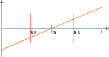
A message reception is considered in time, if it is received within the timeliness interval. If it is received outside the timeliness interval, the message reception is considered invalid. This is related to the communication error "unacceptable deviation from target end-to-end latency" (see subclause B.6). In other words, maximum end-to-end latency = tUB and minimum end-to-end latency = tLB.
Timeliness is related to deviation (see subclause C.4.4), the lower bound tLB is related to earliness (see subclause C.4.5), and the upper bound tUB is related to lateness (see subclause C.4.6).
C.4.4 Deviation p. 91
The term deviation describes the discrepancy between an actual value (tA) and a tArget value (tR).
Deviation(tA) = tA - tR.
Figure C.4.4-1 shows two examples. The tArget value is 10 time units (tR = 10) in both cases. In the first case (blue) the actual value measures 12 time units (tA = 12). The difference of both amounts to +2 time units, which means that the deviation is 2 time units [Accurracy(tA) = 2]. The second case (purple) shows the actual value as 9 time units (tA = 9). The difference of both amounts to -1 time unit, which means that the deviation is -1 time units [Accuracy(tA) = -1].
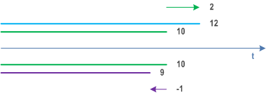
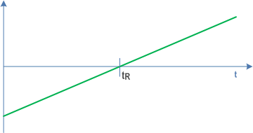
Figure C.4.4-2 shows the deviation with respect to the tArget time (t). The following applies:
Deviation(t) < 0 for t < tR; that is, the arrival is early.
Deviation(t) = 0 for t = tR; that is, the arrival is as desired, i.e. on time.
Deviation(t) > 0 for t > tR; that is, the arrival is late (see also clause C.4.6)
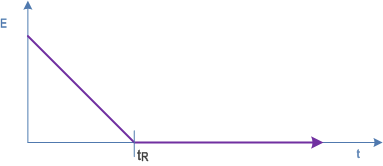
C.4.5 Earliness p. 92
Earliness describes how early the actual value is: earliness is greater than 0 if the actual value is less than the tArget value (see Figure C.4.5-1). The following applies:
Earliness(tA) = tR - tA = -Deviation(tA) for tA < tR;
Earliness(tA) = 0 for tA ≥ tR.
In an example, the tArget value is 10 time units (tR = 10), and the actual value is 7 time units (tA = 7). The difference of both is 3 time units with respect to being early. That means that the earliness is 3 time units [Earliness(tA) = 3].
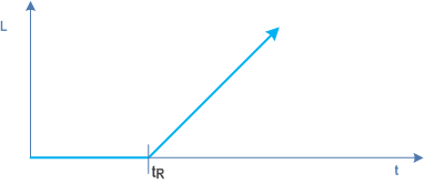
C.4.6 Lateness p. 93
Lateness describes how much greater the actual value is than the tArget value: lateness is greater than 0 if the actual value is greater than the desired value (see Figure C.4.6-1). The following applies:
L(tA) = 0 for tA ≤ tR;
L(tA) = tA-tR = Deviation(tA) for tA > tR.
In an example, the tArget value is 10 time units (tR = 10), and the actual value measures 14 time units (tA = 14). The difference of both is 4 time units with respect to being late. That means that the lateness is 4 time units [L(tA) = 4].
C.4.7 Conclusion p. 93
Using the concepts of earliness and lateness (see subclause C.4.5 and subclause C.4.6, respectively), the maximum and minimum end-to-end latency can be rewritten as follows.
Maximum end-to-end latency = target end-to-end latency + maximum lateness;
Minimum end-to-end latency = target end-to-end latency - maximum earliness.
![]()
![]()
![]()