Content for TS 26.114 Word version: 18.9.0
0…
3…
4…
5…
6…
6.2.3…
6.2.5…
6.2.7…
6.2.10…
7…
7.5…
8…
9…
10…
10.2.1.6…
10.2.2…
10.3…
10.4…
11…
12…
12.3…
12.7…
13a…
16…
16.5…
17…
18…
19…
A…
A.3…
A.4…
A.5…
A.10…
A.14…
A.15…
B…
C…
C.1.3…
C.1.3.5
C.2…
D
E…
E.18…
E.31…
G…
K…
L…
M…
N…
O…
P…
P.3
Q…
R…
S…
T…
U…
V…
W…
X…
Y…
Y.6…
Y.6.4…
Y.6.5…
Y.7…
C.1.3 Adaptation state machine implementations
C.1.3.1 General
C.1.3.2 Adaptation state machine with four states
C.1.3.3 Adaptation state machine with four states (simplified version without frame aggregation)
C.1.3.4 Adaptation state machine with two states
...
...
C.1.3 Adaptation state machine implementations p. 327
C.1.3.1 General p. 327
The example adaptation state machines shown in this section are different realizations of the control algorithm for the adaptation requests. Note that this does not include how the actual signalling should be done but how various triggers will result in the transmission of different requests.
The example adaptation state machines make use of the signalling state machine outlined in clause B.2. Common to all adaptation state machines is that it is possible to implement all versions in the same code and just exclude appropriate states depending on desired mode of operation. All examples can transit between a number of states (denoted S1…S4). In these examples, it is assumed that the codec is AMR-NB and that it uses two coding rates (AMR 12.2 and AMR 5.9). However, this is not a limitation of the adaptation mechanism by itself. It is only the scenario used in these examples.
Since the purpose of the adaptation mechanism is to improve the quality of the session, any adaptation signalling is based upon some trigger; either a received indication or a measurement. In the case of a measurement trigger, it is important to gather reliable statistics. This requires a measurement period which is sufficiently long to give a reliable estimation of the channel quality but also sufficiently short to enable fast adaptation. For typical MTSI scenarios on 3GPP accesses, a measurement period in the order of 100 packets is recommended. Further, in order to have an adaptation control which is reliable and stable, a hangover period is needed after a new state has been entered (typically 100 to 200 packets). An even longer hangover period is suitable when transiting from an error resilient state or a reduced rate into the default, normal state. In the below examples, it is assumed that the metric used in the adaptation is the packet loss rate measured on the application layer. It is possible to use other metrics such as lower layer channel quality metrics.
The example solution is designed based on the following assumptions:
-
When the packet loss rate increases, the adaptation should:
- First try with a lower codec mode rate, i.e. bit-rate back off.
- If this does not improve the situation, then one should try with packet rate back-off by increasing the frame aggregation.
- If none of these methods help, then application layer redundancy should be added to save the session.
- When the packet loss rate increases, one should try to increase the bit rate in a "safe" manner. This is done by probing for higher bit rates by adding redundancy.
- The downwards adaptation, towards lower rates and redundancy, should be fast while the upwards adaptation should be slow.
- Hysteresis should be used to avoid oscillating behaviour between two states.
| State | Description |
|---|---|
| S1 | Default/normal state: Good channel conditions.
This state has the properties:
|
| S2 | In this state the encoding bit-rate and the packet rate is reduced. The state is divided into 2 sub states (S2a and S2b). In state S2a the codec rate is reduced and in state S2b the packet rate is also reduced (the frame aggregation is increased). State S2a may also involve a gradual decrease of the codec-rate in order to be in agreement with the session parameters. If no restrictions are in place regarding mode changes (i.e. such as only allowing changing to a neighbouring mode), it changes bit-rate to the target reduced bit-rate directly. If restrictions are in place, several mode changes might be needed.
This state has the properties:
|
| S3 | This is an interim state where the total bit-rate and packet rate is roughly equal to state S1. 100% redundancy is used with a lower codec mode than S1. This is done to probe the channel band-width with a higher tolerance to packet loss to determine if it is possible to revert back to S1 without significantly increase the packet loss rate.
This state has the properties:
|
| S4 | In this state the encoding bit-rate is reduced (the same bit-rate as in S2) and redundancy is turned on. Optionally also the packet rate is kept the same as in state S2.
This state has the properties:
|
The parameters and other definitions controlling the behaviour of the adaptation state machine are described in Table C.4. Example values are also shown, values which give good performance on a wide range of different channel conditions.
| Parameter | Value/meaning | Comment |
|---|---|---|
| PLR_1 | 3 % | |
| PLR_2 | 1 % | |
| PLR_3 | 2 % | |
| PLR_4 | 10 % | |
| N_INHIBIT | 1 000 frames | A random value may be used to avoid large scale oscillation problems. |
| N_HOLD | 5 measurement periods | |
| T_RESPONSE | 500 ms | Estimated response time for a request to be fulfilled. |
| Packet loss burst | 2 or more packet losses in the last 20 packets. |
As described in Annex C.1.1, the frame loss rate (FLR) can be used instead of the packet loss rate to trigger the adaptation. The benefit with using FLR is that this metric can (and should) include the late losses that occur if frames are received too late to be useful for decoding. Table C.4a shows thresholds that can be used for FLR if the FLR-triggered adaptation is used instead of the PLR-triggered adaptation.
| Parameter | Value/meaning | Comment |
|---|---|---|
| FLR_1 | 3 % | Used instead of PLR_1 |
| FLR_2 | 1 % | Used instead of PLR_2 |
| FLR_3 | 2 % | Used instead of PLR_3 |
| FLR_4 | 3 % | Used instead of PLR_4 |
| Frame loss burst | 2 or more frame losses in the last 20 frames. | Replaces packet loss burst |
The adaptation state machines shown in Annex C.1.3.2, C.1.3.3 and C.1.3.4 can be used also for FLR-triggered adaptation by applying the following modifications:
- The media receiver needs to measure the frame loss rate instead of the packet loss rate. The frame loss rate includes late losses.
- The PLR thresholds need to be replaced with the corresponding FLR thresholds, as shown in Table C.4a.
C.1.3.2 Adaptation state machine with four states p. 329
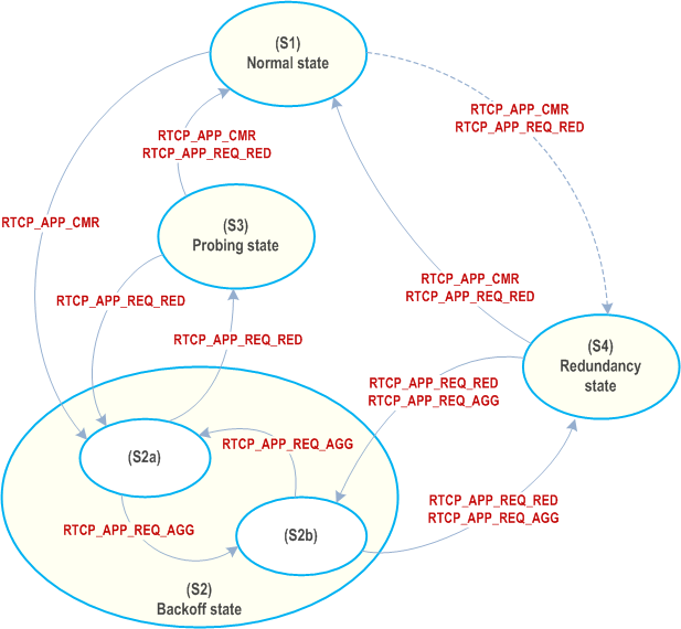
The first example utilizes all adaptation possibilities, both in terms of possible states and transitions between the states. Figure C.2 shows the layout of the adaptation state machine and the signalling used in the transitions between the states.

State transitions:
Below are listed the possible state transitions and signalling that is involved. Note that the state can go from S1 to either S2 or state S4, this is explained below:
| State transition | Conditions and actions |
|---|---|
| S1 → S2a | Condition: Packet loss ≥ PLR_1 or packet loss burst detected. A request to reduce the encoding bit-rate is sent using RTCP_APP_CMR, e.g. change mode from AMR 12.2 to AMR 5.9. |
| S2a → S2b | Condition: Packet loss ≥ PLR_1. This state transition occurs if the packet loss is still high despite the reduction in codec rate. A request is sent to reduce the packet rate is reduced by means of an RTCP_APP_REQ_AGG message. |
| S2b → S2a | Condition: Packet loss ≤ PLR_ 2 for N_HOLD consecutive measurement periods. This state transition involves an increase of the packet rate restoring it to the same value as in S1. The request transmitted is RTCP_APP_REQ_AGG. If the state transition S2b→S2a→S2b occurs in sequence, the state will be locked to S2b for N_INHIBIT frames to avoid state oscillation. |
| S2a → S3 | Condition: Packet loss ≤ PLR_2 for N_HOLD consecutive measurement periods. A request to turn on 100% redundancy is transmitted by means of request RTCP_APP_REQ_RED. |
| S3 → S2a | Condition: Packet loss ≥ PLR_3. Same actions as in transition from, S1→S2a. If the transition S2a→S3→S2a→S3→S2a occurs, the S3 is disabled for N_INHIBIT frames. |
| S3 → S1 | Condition: Packet loss ≤ PLR_2 for N_HOLD consecutive measurement periods. A request to turn off redundancy is transmitted as RTCP_APP _REQ_RED. Encoding bit-rate is increased by means of RTCP_APP_CMR. |
| S2b → S4 | Condition: Packet loss ≥ PLR_3. A request to turn on 100% redundancy is transmitted by means of request RTCP_APP_REQ_RED. The packet rate is restored to same value as in S1 using RTCP_APP _REQ_AGG. |
| S4 → S2b | Condition:
|
| S4 → S1 | Condition: Packet loss < PLR_3 for N_HOLD consecutive measurement periods. A request to turn off redundancy is transmitted using RTCP_APP _REQ_RED. Encoding bit-rate is requested to increase using RTCP_APP_CMR. |
| S1 → S4 | Condition: Packet loss ≥ PLR_1 or packet loss burst detected AND the previous transition was S4→S1, otherwise the transition S1→S2a will occur. A request to turn on 100% redundancy is transmitted using RTCP_APP_REQ_RED. The encoding bit-rate is requested to be reduced (in the example from AMR 12.2 to AMR 5.9) using RTCP_APP_CMR. |
C.1.3.3 Adaptation state machine with four states (simplified version without frame aggregation) p. 332
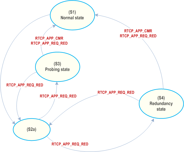
This example is a simpler implementation with the frame aggregation removed.

State transitions:
Below are listed the possible state transitions and signalling that is involved.
| State transition | Conditions and actions |
|---|---|
| S1 → S2a | Condition: Packet loss ≥ PLR_1 or packet loss burst detected. A request to reduce the encoding bit-rate is sent using RTCP_APP_CMR, e.g. change mode from AMR 12.2 to AMR 5.9. |
| S2a → S3 | Condition: Packet loss ≤ PLR_2 for N_HOLD consecutive measurement periods. A request to turn on 100% redundancy is transmitted by means of request RTCP_APP_REQ_RED. |
| S3 → S2a | Condition: Packet loss ≥ PLR_3. Same actions as in transition from, S1→S2a. If the transition S2a→S3→S2a→S3→S2a happens in sequence state S3 is disabled for N_INHIBIT frames. |
| S3 → S1 | Condition: Packet loss ≤ PLR_2 for N_HOLD consecutive measurement periods. A request to turn off redundancy is transmitted as RTCP_APP _REQ_RED. Encoding bit-rate is increased by means of RTCP_APP_CMR. |
| S2a → S4 | Condition: Packet loss ≥ PLR_3. A request to turn on 100% redundancy is transmitted by means of request RTCP_APP_REQ_RED. |
| S4 → S2a | Condition: Packet loss ≥ to 4*PLR@ S2b→S4 (packet loss considerably increased since transition to state S4). This is indicative of that the total bit-rate is too high and that it is probably better to transmit with a lower packet rate/bit-rate instead. This case might occur if the packet loss is high in S2a due to a congested link, a switch to redundant mode S4 will then increase the packet loss even more. |
| S4 → S1 | Condition: Packet loss < PLR_3 for N_HOLD consecutive measurement periods. A request to turn off redundancy is transmitted using RTCP_APP _REQ_RED. Encoding bit-rate is requested to increase using RTCP_APP_CMR. |
C.1.3.4 Adaptation state machine with two states p. 334
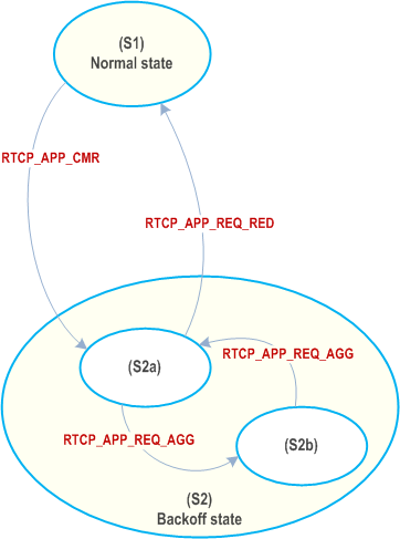
This example is an implementation with the redundant states removed.

State transitions:
Below are listed the possible state transitions and signalling that is involved.
| State transition | Conditions and actions |
|---|---|
| S1 → S2a | Condition: Packet loss ≥ PLR_1 or packet loss burst detected. A request to reduce the encoding bit-rate is sent using RTCP_APP_CMR, e.g. change mode from AMR 12.2 to AMR 5.9. A failed transition counter counts the number of consecutive switching attempts S2a→S1 that fails. In the number of failed attempts is two or more state S1 is inhibited for N_INHIBIT frames. A failed transition attempt occurs if the previous transition was S2a→S1 and the state transition immediately occurs back to S2a. |
| S2a → S2b | Condition: Packet loss ≥ PLR_1. This state transition occurs if the packet loss is still high despite the reduction in codec rate. A request is sent to reduce the packet rate is reduced by means of an RTCP_APP_REQ_AGG message. |
| S2b → S2a | Condition: Packet loss ≤ PLR_2 for N_HOLD consecutive measurement periods. This state transition involves an increase of the packet rate. Also packet rate is restored to same value as in State (1) RTCP_APP_REQ_AGG. If the state transition S2b→S2a→S2b occurs in sequence, the state will be locked to S2b for N_INHIBIT frames. |
| S2a → S1 | Condition: Packet loss ≤ PLR_2 for N_HOLD consecutive measurement periods. Redundancy is turned on (100%) by means of request RTCP_APP_REQ_RED. |